Exercise Solution for Chapter 6
Chapter 6, Exercise 6.4
Make a less extreme example of correlated test statistics than the data duplication at the end of Section 6.5. Simulate data with true null hypotheses only, and let the data morph from having completely independent replicates (columns) to highly correlated as a function of some continuous-valued control parameter. Check type-I error control (e.g., with the p-value histogram) as a function of this control parameter.
We’ll go through a few data clean up and exploration steps first, then we’ll walk through the code related specifically to the exercise a little further down in the post.
library(tidyverse)
library(purrr)
library(ggbeeswarm)
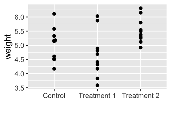
For this exercise we use the PlantGrowth dataset from the datasets package in R. The dataset includes results from an experiment on plant growth comparing yields (as measured by dried weight of plants) obtained under a control and two different treatment conditions.
data("PlantGrowth")
head(PlantGrowth)
## weight group
## 1 4.17 ctrl
## 2 5.58 ctrl
## 3 5.18 ctrl
## 4 6.11 ctrl
## 5 4.50 ctrl
## 6 4.61 ctrlHere we’re plotting the outcomes of the three groups (ctrl, trt1, and trt2):
PlantGrowth %>%
   mutate(group = fct_recode(group,
                            Control = "ctrl",
                            `Treatment 1` = "trt1",
                            `Treatment 2` = "trt2")) %>%
  ggplot(aes(x = group, y = weight)) +
  geom_beeswarm() +
  labs(x = "")
Often in research one of the simplest comaparisons of data we can make is between two groups. The t-test is one of the many statistics used in hypothesis testing and can help us determine if the differences between two group means is “significant” or if the differences could have happened by chance. The test statistic is defined as:
\(t=\frac{\bar{m_1}-\bar{m_2}}{\sqrt{s_1^2/N_1 + s_2^2/N_2}}\)
where \(\bar{m_1}\) and \(\bar{m_2}\) are the sample means in group 1 and 2, respectively, which have \(N_1\) and \(N_2\) observations each, and \(s_1\) and \(s_2\) are the sample variances for each of the two groups.
Next we’ll apply a t-test comparing weights in the ctrl group to the trt2 group. We’re testing against the null hypothesis that there is no difference in mean dried plant weights between the two groups.
PlantGrowth %>%
  filter(group %in% c("ctrl", "trt2")) %>%
    t.test(weight ~ group, data  = .)
##
## Welch Two Sample t-test
##
## data: weight by group
## t = -2.134, df = 16.786, p-value = 0.0479
## alternative hypothesis: true difference in means is not equal to 0
## 95 percent confidence interval:
## -0.98287213 -0.00512787
## sample estimates:
## mean in group ctrl mean in group trt2
## 5.032 5.526Here’s the tidy version:
library("broom")
(ttest_orig <- PlantGrowth %>%
  filter(group %in% c("ctrl", "trt2")) %>%
  t.test(weight ~ group, data  = .) %>%
    tidy())
## # A tibble: 1 x 10
## estimate estimate1 estimate2 statistic p.value parameter conf.low conf.high
## <dbl> <dbl> <dbl> <dbl> <dbl> <dbl> <dbl> <dbl>
## 1 -0.494 5.03 5.53 -2.13 0.0479 16.8 -0.983 -0.00513
## # … with 2 more variables: method <chr>, alternative <chr>Then we’ll duplicate the data, adding a second copy of the dataframe, before running the t-test.
(ttest_dup <- PlantGrowth %>%
  bind_rows(PlantGrowth) %>% # Add the duplicate of the dataset
  filter(group %in% c("ctrl", "trt2")) %>%
  t.test(weight ~ group, data  = .) %>%
  tidy())
## # A tibble: 1 x 10
## estimate estimate1 estimate2 statistic p.value parameter conf.low conf.high
## <dbl> <dbl> <dbl> <dbl> <dbl> <dbl> <dbl> <dbl>
## 1 -0.494 5.03 5.53 -3.10 0.00377 35.4 -0.817 -0.171
## # … with 2 more variables: method <chr>, alternative <chr>Notice that the p-value is smaller (now less than 0.05) even though the group means haven’t changed. This is due solely to the increase in sample size.
However, we’ve violated the t-test assumption of independence. Paired (in this case blatantly duplicated) data is dependent and would be more appropriately tested by a two-sample paired test. A similar example with experimental data would involve taking duplicate measures (technical replicates) on 15 subjects (e.g., leaf, mouse, human) and assuming you now have 30 independent measurements; that would be incorrect. Taking repeated measurements on 15 subjects would leave you with just 15 independent measurments (and the other 15 fully dependent on those).
If the data sampled for a t-test violates one or more of the t-test assumptions, such as independence or normal distribution, results can be incorrect and misleading.
Next we resample only half the data and then duplicated that sampled half to create a datset; so the size of the data set is the same as the original dataset (n = 30), but now half of the observations are fully dependent (exactly the same) as other observations in the dataset.
The purpose of the set.seed function is to set the seed of R’s random number generator. We use it below in our simulations so that the results of our sampled data don’t change each time the document is re-rendered and therefore can be reproduced.
set.seed(4234)

pg1 <- PlantGrowth %>%
  sample_frac(size = 0.5) %>%
  bind_rows(., .)

(pg1_ttest <- pg1 %>%
  filter(group %in% c("ctrl", "trt2")) %>%
  t.test(weight ~ group, data  = .) %>%
  tidy())
## # A tibble: 1 x 10
## estimate estimate1 estimate2 statistic p.value parameter conf.low conf.high
## <dbl> <dbl> <dbl> <dbl> <dbl> <dbl> <dbl> <dbl>
## 1 -0.492 5.23 5.72 -1.98 0.0722 11.3 -1.04 0.0524
## # … with 2 more variables: method <chr>, alternative <chr>The p-value increases from 0.004 with a fully duplicated dataset to a value typically much higher with half the data duplicated.
As discussed in section 6.5 of the text, the t-test function uses asymptotic theory to compute the t-statistic: “this theory states that under the null hypothesis of means in both groups, the statistic follows a known, mathematical distribution, the so called t-distribution with \(n^1 + n^2\) degrees of freedom” As we’ve discussed above, the theory also makes the assumption of independence, normality, and equal variance.
There are often variations from these assumptions in real world data. In our plant growth example, weights are always positive while the normal distribution spans over the entire axis.
Below we use permutation tests to assess whether the deviation from theoretical assumptions makes a difference. We first use replicate to
run a lot of t-tests where we test our original data, but with the
group column randomly re-ordered, so any true relationship between
the group and weight measurements is broken:
pg1_null = with(
  dplyr::filter(pg1, group %in% c("ctrl", "trt2")),
    replicate(10000,
      abs(t.test(weight ~ sample(group))$statistic)))

# You can see that this results in a long vector of t statistic
# values, each estimated from a version of the data where we
# randomized the group labels
head(pg1_null)
## t t t t t t
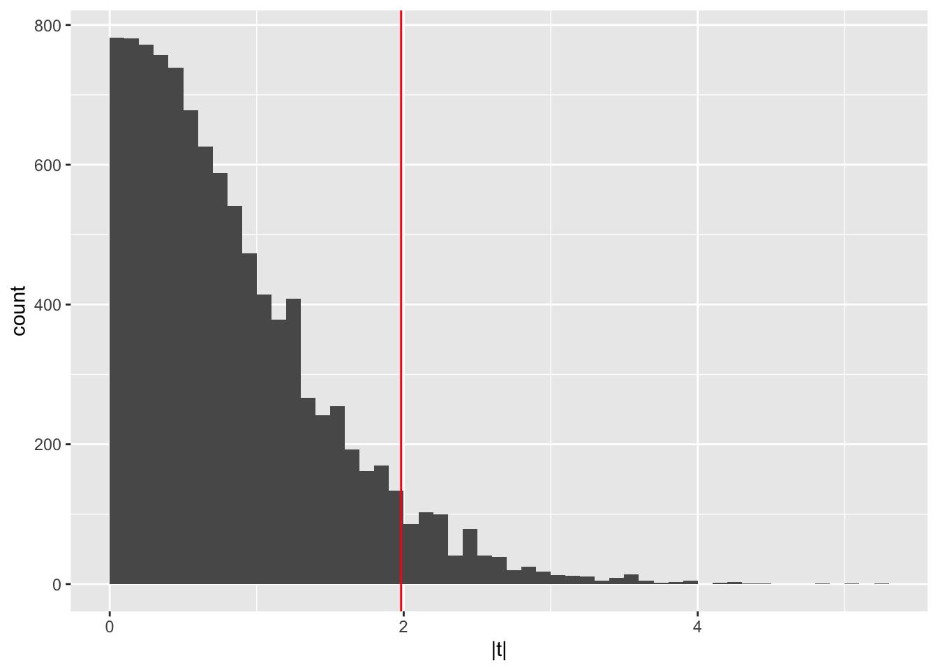
## 0.5065581 0.9543497 0.5703743 0.5760347 0.5101952 1.6371872These should represent the pattern of how t statistics for this
data would be distributed under the null hypothesis that there is no
difference between the average weights of the two groups.
We can plot a histogram of all these t statistic values to visualize
the distribution of the t statistic under the null hypothesis, adding
a line to show the t statistic we observed in the real data (without
shuffling the group column):
ggplot(tibble(`|t|` = pg1_null), aes(x = `|t|`)) +
  geom_histogram(binwidth = 0.1, boundary = 0) +
  geom_vline(xintercept = abs(pg1_ttest$statistic), col = "red")
In general, a permutation test is a type of statistical significance test in which the distribution of the test statistic under the null hypothesis is obtained by calculating all possible values of the test statistic under all possible rearrangements of the observed data points (https://wikipedia.org).
The test essentially exchanges labels between samples and what they measure; if the connections between label and measurements are broken our t-test should show no connection between the two, demonstrating a true null hypothesis that there is no difference between group means.
Now we’ll take the dataset with half resampled, and add random noise to each observation.
set.seed(1234)

pg2 <- pg1 %>%
  mutate(noise = rnorm(30, mean = 0, sd = 0.2),
         weight = weight + noise) %>%
  select(-noise)
head(pg2)
## weight group
## 1 5.908587 trt2
## 2 6.165486 ctrl
## 3 6.526888 trt2
## 4 4.030860 ctrl
## 5 4.775825 trt1
## 6 5.241211 ctrl(pg2_ttest <- pg2 %>%
filter(group %in% c("ctrl", "trt2")) %>%
t.test(weight ~ group, data = .) %>%
tidy())## # A tibble: 1 x 10
## estimate estimate1 estimate2 statistic p.value parameter conf.low conf.high
## <dbl> <dbl> <dbl> <dbl> <dbl> <dbl> <dbl> <dbl>
## 1 -0.562 5.14 5.70 -1.97 0.0767 10.3 -1.20 0.0721
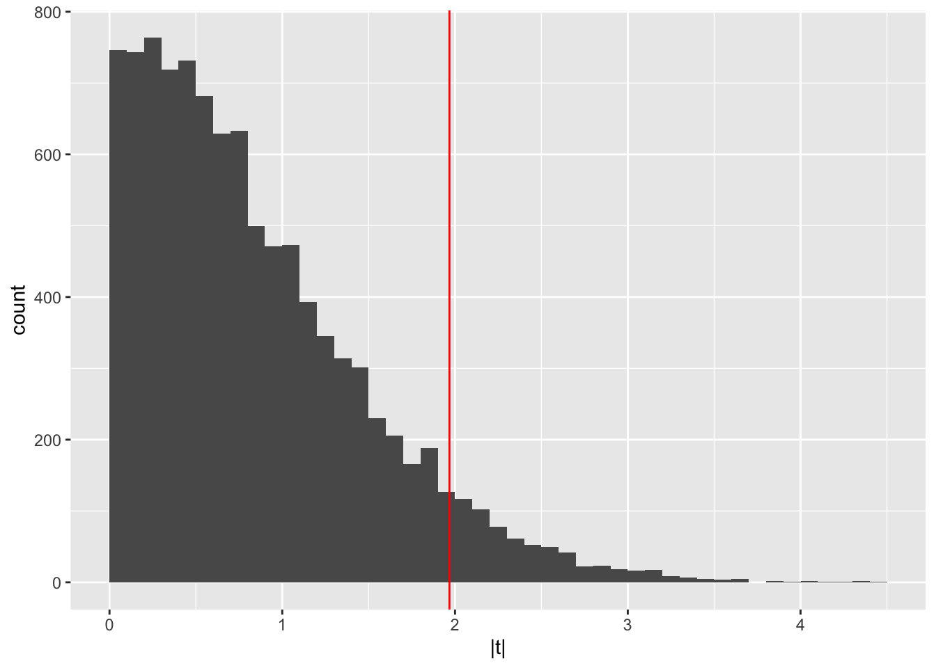
## # … with 2 more variables: method <chr>, alternative <chr>Permutation test data with half duplicated and random noise added:
pg2_null = with(
  dplyr::filter(pg2, group %in% c("ctrl", "trt2")),
    replicate(10000,
      abs(t.test(weight ~ sample(group))$statistic)))

head(pg2_null)
## t t t t t t
## 0.63521740 1.71201809 0.73541313 0.61678119 0.02298951 1.38779279ggplot(tibble(`|t|` = pg2_null), aes(x = `|t|`)) +
geom_histogram(binwidth = 0.1, boundary = 0) +
geom_vline(xintercept = abs(pg2_ttest$statistic), col = "red") 
If the t-test statistic we see in our permutation test looks different compared to our observed data then we can most likely conclude that our data was not generated under the null hypothesis of no significant difference between the treatment groups. We would therefore reject the null hypothesis.
The table below summarizes the four different types of datasets we’ve explored with t-tests. Important to note is that all of these results are from random samples; the exact p-values and test statistics are variable and if someone were to run a code with a different seed, they would get different results.
library(kableExtra)

data_summary <- bind_rows(ttest_orig, ttest_dup,
                          pg1_ttest, pg2_ttest) %>%
  mutate(data = c('original',
                  'doubled without random noise',
                  'same size as original, half observations replicated',
                  'half replicated, random noise added to each replicate'),
         n = c(30, 60, 30 ,30)) %>%
  select(data, n, statistic, p.value)

data_summary %>%
   kable(align = c("l")) %>%
  kable_styling(bootstrap_options = c("striped", "hover",
                                      "condensed")) %>%
  column_spec(1, bold = T, border_right = T) %>%
column_spec(2:3, width = "6em")| data | n | statistic | p.value |
|---|---|---|---|
| original | 30 | -2.134021 | 0.0478993 |
| doubled without random noise | 60 | -3.100660 | 0.0037738 |
| same size as original, half observations replicated | 30 | -1.982154 | 0.0722163 |
| half replicated, random noise added to each replicate | 30 | -1.967597 | 0.0766878 |