Exercise 2.3 from Modern Statistics for Modern Biologists

A sequence of three nucleotides codes for one amino acid. There are 4 nucleotides, thus \(4^3\) would allow for 64 different amino acids, however there are only 20 amino acids requiring only 20 combinations + 1 for an “end” signal. (The “start” signal is the codon, ATG, which also codes for the amino acid methionine, so the start signal does not have a separate codon.) The code is redundant. But is the redundancy even among codons that code for the same amino acid? In other words, if alanine is coded by 4 different codons, do these codons code for alanine equally (each 25%), or do some codons appear more often than others? Here we use the tuberculosis genome to explore codon bias.

a) Explore the data, mtb

Use table to tabulate the AmAcid and Codon variables.

Each amino acid is encoded by 1–6 tri-nucleotide combinations.

mtb = read.table("example_datasets/M_tuberculosis.txt", header = TRUE)
codon_no <- rowSums(table(mtb))
codon_no

## Ala Arg Asn Asp Cys End Gln Glu Gly His Ile Leu Lys Met Phe Pro Ser Thr Trp Tyr 
##   4   6   2   2   2   3   2   2   4   2   3   6   2   1   2   4   6   4   1   2 
## Val 
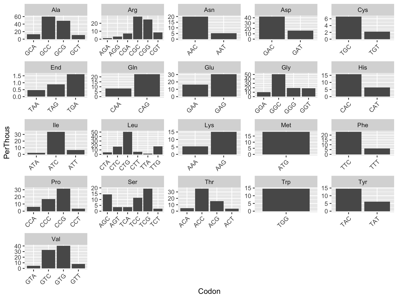
##   4

The PerThousands of each codon can be visualized, where each plot represents an amino acid and each bar represents a different codon that codes for that amino acid. But what does the PerThousands variable mean?

ggplot(mtb, aes(x=Codon, y=PerThous)) +
  geom_col()+
  facet_wrap(~AmAcid, scales="free") +
  theme(axis.text.x = element_text(angle = 45, hjust = 1))

b) The PerThous variable

How was the PerThous variable created?

The sum of all of the numbers of codons gives you the total number of codons in the M. tuberculosis genome: all_codons. Remember that this is not the size of the M. tuberculosis genome, but the number of codons in all M. tuberculosis genes. To get the size of the genome, multiply each codon by 3 (for each nucleotide) and add all non-coding nucleotides (which we do not know from this data set).

all_codons = sum(mtb$Number)
all_codons

## [1] 1344223

The PerThousands variable is derived by dividing the number of occurrences of the codon of interest by the total number of codons. Because this number is small and hard to interpret, multiplying it by 1000 gives a value that is easy to make sense of. Here is an example for proline. The four values returned align to the four codons that each code for proline.

pro  =  mtb[mtb$AmAcid == "Pro", "Number"]
pro / all_codons * 1000

## [1] 31.560240  6.121752  3.405685 17.032144

c) Codon bias

Write an R function that you can apply to the table to find which of the amino acids shows the strongest codon bias, i.e., the strongest departure from uniform distribution among its possible spellings.

First, let’s look at the expected frequencies of each codon.

codon_expected <- data.frame(codon_no) %>%
  rownames_to_column(var = "AmAcid") %>%
  mutate(prob_codon = 1/codon_no)
codon_expected

##    AmAcid codon_no prob_codon
## 1     Ala        4  0.2500000
## 2     Arg        6  0.1666667
## 3     Asn        2  0.5000000
## 4     Asp        2  0.5000000
## 5     Cys        2  0.5000000
## 6     End        3  0.3333333
## 7     Gln        2  0.5000000
## 8     Glu        2  0.5000000
## 9     Gly        4  0.2500000
## 10    His        2  0.5000000
## 11    Ile        3  0.3333333
## 12    Leu        6  0.1666667
## 13    Lys        2  0.5000000
## 14    Met        1  1.0000000
## 15    Phe        2  0.5000000
## 16    Pro        4  0.2500000
## 17    Ser        6  0.1666667
## 18    Thr        4  0.2500000
## 19    Trp        1  1.0000000
## 20    Tyr        2  0.5000000
## 21    Val        4  0.2500000

Next, calculate the observed frequencies for each codon seen in the data set and use the chi-squared test statistic to determine if the difference between expected and observed codon frequencies is even or if some codon sequences are used more than others.

To start, you can group the data by amino acid and then determine a few things about the amino acid or the possible codons for it, including the total observations across all codons for the amino acid (total), the number of codons for that amino acid (n_codons), and the expected count for each codon for that amino acid (the total number of observations for that amino acid divided by the number of codons, giving an expected number that’s the same for all codons of an amino acid; expected).

codon_compared <- mtb %>% 
  group_by(AmAcid) %>% 
  mutate(total = sum(Number),
         n_codons = n(),
         expected = total / n_codons)
codon_compared

## # A tibble: 64 x 7
## # Groups:   AmAcid [21]
##    AmAcid Codon Number PerThous  total n_codons expected
##    <fct>  <fct>  <int>    <dbl>  <int>    <int>    <dbl>
##  1 Gly    GGG    25874    19.2  132810        4   33202.
##  2 Gly    GGA    13306     9.9  132810        4   33202.
##  3 Gly    GGT    25320    18.8  132810        4   33202.
##  4 Gly    GGC    68310    50.8  132810        4   33202.
##  5 Glu    GAG    41103    30.6   62870        2   31435 
##  6 Glu    GAA    21767    16.2   62870        2   31435 
##  7 Asp    GAT    21165    15.8   77852        2   38926 
##  8 Asp    GAC    56687    42.2   77852        2   38926 
##  9 Val    GTG    53942    40.1  114991        4   28748.
## 10 Val    GTA     6372     4.74 114991        4   28748.
## # … with 54 more rows

The mutate function is used after group_by to do all this within each amino acid group of codons, but without collapsing to one row per amino acid, as a summarize call would.

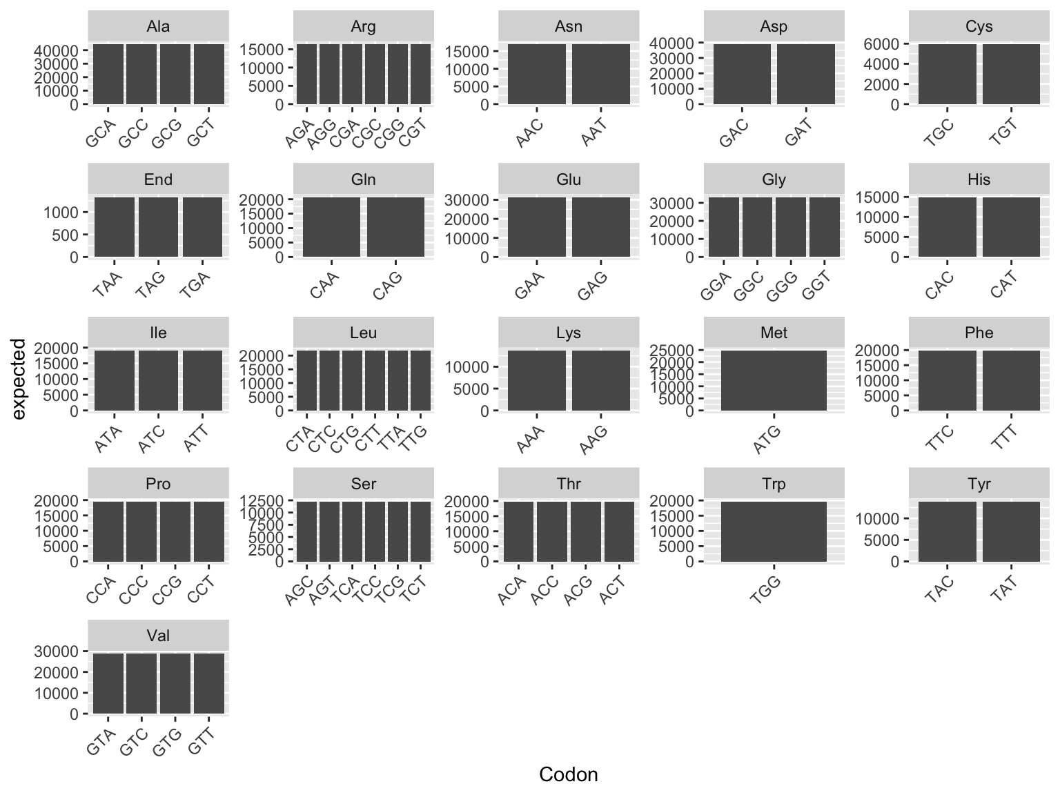
To convince yourself that this has worked out correctly, you can repeat the plot we made before and see that the bars for the expected values are always equal across all codons for an amino acid:

ggplot(codon_compared, aes(x=Codon, y=expected)) +
     geom_col()+
     facet_wrap(~AmAcid, scales="free") +
     theme(axis.text.x = element_text(angle = 45, hjust = 1))

Finally, we can calculate the chi-squared (\(\chi^2\)) statistic and compare it to the chi-squared distribution to get the p-value when testing against the null hypothesis that the amino acid observations are uniformly distributed across codons. The \(\chi^2\) is calculated as:

\[ \chi^2 = \sum_i{\frac{(O_i-E_i)^2}{E_i}} \]

where:

• \(O_i\) is the observed value of data point \(i\) (Number in our data); and
• \(E_i\) is the expected value of data point \(i\) (expected in our data)

In our data, we can calculate the contribution to the total \(\chi^2\) statistic from each data point (in this case, each codon within an amino acid) using mutate, and then add these values up using group_by to group by amino acid followed by summarize to sum up across all the data points for an amino acid. The other information we need to get is the number of codons for the amino acid, because we’ll need this to determine the degrees of freedom for the chi-squared distribution. Next, we used mutate with pchisq to determine the p-values within each amino acid group for the test against the null that the codons are uniformly distributed for that amino acid (i.e., that there isn’t codon bias). These p-values turn out to be super small, so we’re using a technique to get the log-transform versions of them instead, which we explain a bit more later. Finally, we used arrange to list the amino acids by evidence against uniform distribution of the codons, from most evidence against (smallest p-value so most negative log(p-value)) to least evidence against (although still plenty of evidence against) and added an index with the ranking for each codon by adding a column with the sequence of numbers from 1 to the number of rows in the data (n()).

codon_compared %>% 
  filter(n_codons > 1) %>% 
  group_by(AmAcid) %>% 
  mutate(chi_squared = ((Number - expected)^2/expected)) %>% 
  summarise(chi_squared = sum(chi_squared),
            n = n()) %>% 
  mutate(p_value = pchisq(chi_squared, df = n-1, log = TRUE, lower.tail = FALSE)) %>% 
  arrange(p_value) %>% 
  mutate(rank = 1:n())

## # A tibble: 19 x 5
##    AmAcid chi_squared     n p_value  rank
##    <fct>        <dbl> <int>   <dbl> <int>
##  1 Leu        135432.     6 -67700.     1
##  2 Ala         75620.     4 -37805.     2
##  3 Arg         72183.     6 -36076.     3
##  4 Thr         58767.     4 -29378.     4
##  5 Val         58737.     4 -29363.     5
##  6 Ile         56070.     3 -28035.     6
##  7 Gly         52534.     4 -26262.     7
##  8 Pro         45400.     4 -22695.     8
##  9 Ser         36742.     6 -18357.     9
## 10 Asp         16208.     2  -8109.    10
## 11 Phe         13444.     2  -6727.    11
## 12 Asn         11404.     2  -5707.    12
## 13 Gln          9376.     2  -4693.    13
## 14 Lys          6382.     2  -3195.    14
## 15 Glu          5947.     2  -2978.    15
## 16 His          5346.     2  -2678.    16
## 17 Tyr          4738.     2  -2373.    17
## 18 Cys          2958.     2  -1483.    18
## 19 End           928.     3   -464.    19

As you may notice, these log transforms of the p-values (which we got rather than untransformed p-values in the pchisq call because we used the option log = TRUE) are large in magnitude and negative (so very tiny once you take the exponent if you re-transformed them to p-values) values. If you tried to calculate the untransformed p-values (and we did!), this number is so small (0.00000000e+00) that it is too small for R—it shows up as exactly zero in R, even though it actually is a very tiny, but still non-zero, number. To get around this issue, we told pchisq to work on these p-values as log transforms, and then we left the p-value as that log-transformed value. A group of numbers that are log transformed will be in the same order as their untransformed versions, so we don’t need to convert back to figure out which amino acid had that smallest p-value. We can just sort the amino acids from most negative to less negative using these log-transformed versions of the p-values. We now have the amino acids ranked from most biased codons (1) to least (19).