Exercise 2.6

The first part of the exercise asks you to:

Choose your own prior for the parameters of the beta distribution. You can do this by sketching it here: https://jhubiostatistics.shinyapps.io/drawyourprior.

After sketching a plot, I chose the parameters to set up a prior: \(\alpha\) = 2.47 and \(\beta\) = 8.5.

Using this prior

Next, the exercise asks you:

Once you have set up a prior, re-analyse the data from Section 2.9.2, where we saw Y = 40 successes out of n = 300 trials.

To be able to use the loglikelihood function from the text, I first needed to redefine it here:

loglikelihood = function(theta, n = 300, k = 40) { ## Function definition from the textbook
  log(choose(n, k)) + k * log(theta) + (n - k) * log(1 - theta)
}

Then, I created a vector of \(\theta\) values between 0 and 1, spaced 0.001 units wide. The plot below shows different possible values of \(\theta\) and the log likelihood for each of these values:

thetas = seq(0, 1, by = 0.001)
plot(thetas, loglikelihood(thetas), xlab = expression(theta),
     ylab = expression(paste("log f(", theta, " | y)")),type = "l")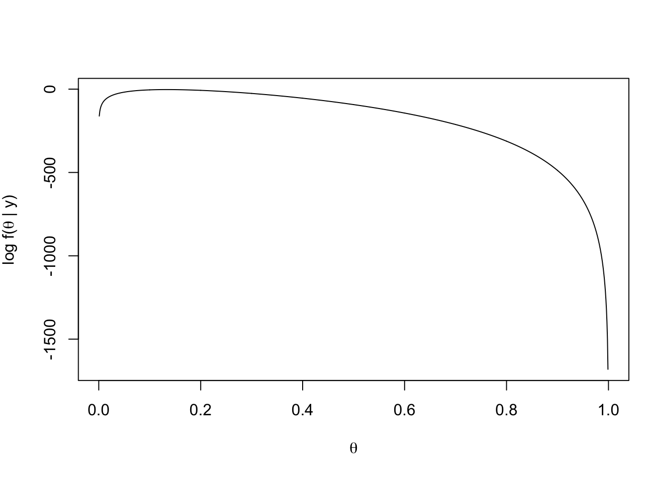

Next, I used rbeta to draw 1,000,000 random samples from a beta distribution with my new picks for the parameters for \(\alpha\) and \(\beta\):

rtheta = rbeta(1000000, shape1 = 2.47, shape2 = 8.5)

After running the above, for each of these \(\theta\) values, we then generate a random sample of \(Y\) as observed in the histogram (with orange bars):

y = vapply(rtheta, function(th) {
  rbinom(1, prob = th, size = 300)
}, numeric(1))
hist(y, breaks = 50, col = "orange", main = "", xlab = "")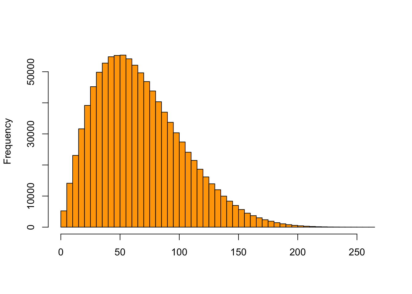

Our next step is to use this information to generate a posterior distribution of \(\theta\) at a fixed \(Y\) value. In this example they used \(Y=40\).

After running the above, for each of these thetas, we generated simulated values for the posterior distribution of \(\theta\) at \(Y=40\) as observed in this histogram (with green bars).

thetaPostEmp = rtheta[ y == 40 ]
hist(thetaPostEmp, breaks = 40, col = "chartreuse4", main = "",
     probability = TRUE, xlab = expression("posterior"~theta), ylim=c(0,40))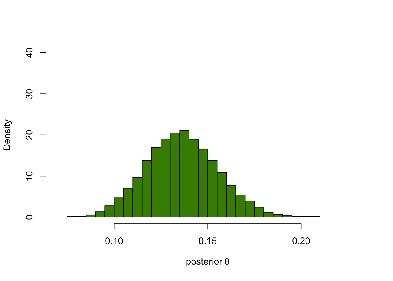

densPostTheory  =  dbeta(thetas, 42.47, 268.5)

You can check how this compares to the theoretical posterior distribution for \(\theta\) at \(Y = 40\):

hist(thetaPostEmp, breaks = 40, col = "chartreuse4", main = "",
  probability = TRUE, xlab = expression("posterior"~theta))
lines(thetas, densPostTheory, type="l", lwd = 3)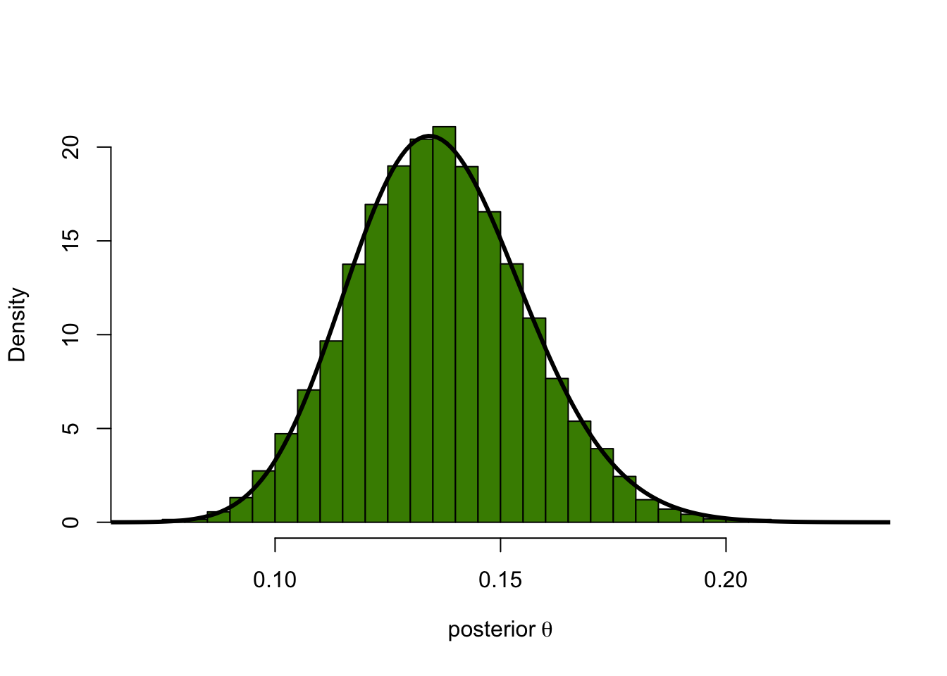

We can also check the means of both distributions computed above.

mean(thetaPostEmp) # Empirical

## [1] 0.1363246

dtheta = thetas[2]-thetas[1]
sum(thetas * densPostTheory * dtheta) # Theoretical

## [1] 0.1365727

thetaPostMC = rbeta(n = 1e6, 42.47, 268.5)
mean(thetaPostMC)

## [1] 0.1365813

qqplot(thetaPostMC, thetaPostEmp, type = "l", asp = 1)
abline(a = 0, b = 1, col = "blue")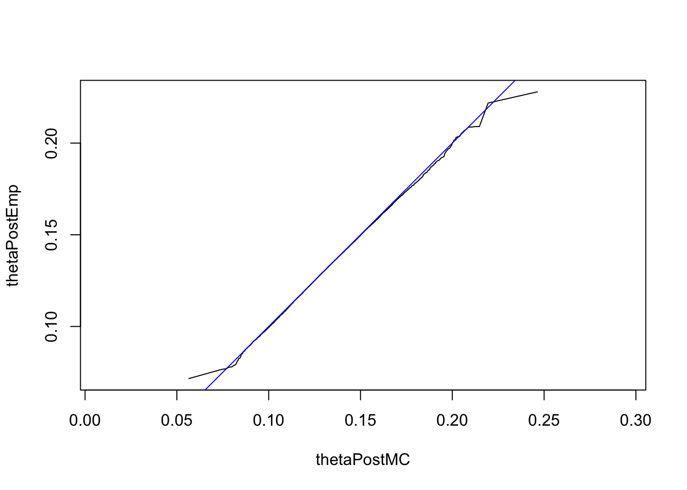

densPost2 = dbeta(thetas, 42.47, 268.5)
mcPost2   = rbeta(1e6, 42.47, 268.5)
sum(thetas * densPost2 * dtheta)  # mean, by numeric integration

## [1] 0.1365727

mean(mcPost2)                     # mean, by MC

## [1] 0.1365487

thetas[which.max(densPost2)]      # MAP estimate

## [1] 0.134

quantile(mcPost2, c(0.025, 0.975))

##      2.5%     97.5% 
## 0.1007321 0.1767921